The Custom Bonding Curve I Didn't Ship

Drafted April 2025. Finished and published August 2026 as part of the migration away from WordPress.

Upside’s first market implementation created an ERC20 token for a piece of content and put its supply into a single-sided Uniswap V3 position. It gave us a working market without having to build an automated market maker (AMM).

When I started moving that market into the protocol contract, I did not begin with the constant-product formula. I built and modelled a bonding curve from scratch.

The idea was to divide supply into one-million-token bands. Price would rise linearly inside each band, then rise more steeply in the next. It looked simple on a chart. Making arbitrary buys and sells agree was where the real engineering started.

A continuous curve made from linear bands

The curve had four rules:

• the first token cost $0.01;
• price doubled for every one million tokens issued;
• there was no price jump at a band boundary; and
• excluding fees and rounding, selling had to retrace buying exactly.

For a supply s, I split the position into a zero-based band number j and an offset u inside that band:

W   = 1,000,000 tokens
j   = floor(s / W)
u   = s mod W

B_j = $0.01 × 2^j
m_j = B_j / W

price(s) = B_j + m_j × u

The first band therefore ran linearly from $0.01 to $0.02. The second ran from $0.02 to $0.04, and the third from $0.04 to $0.08. Both the base price and the slope doubled each time.

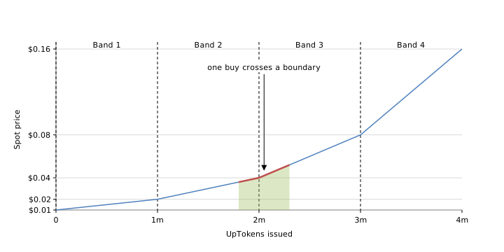
A new band changed the slope, not the price. The end of one line was the start of the next.

This produced something closer to exponential growth while keeping each segment linear. It also gave the protocol predictable milestones: one million tokens moved the price to $0.02, two million to $0.04, and ten million to $10.24.

A quote was an area, not a spot price

The contract could not quote a large order by multiplying the current price by the number of tokens. Every token moved the price. The buyer had to pay the area under the curve.

For n tokens bought from offset u inside one band, the cost was:

cost = n × (B_j + m_j × u) + (m_j × n²) / 2

At the start of a band, where u = 0, buying all one million tokens cost one and a half times the base price multiplied by the band width. The first band cost $15,000. The second cost $30,000. Buying the first ten million tokens cost $15,345,000 in total.

A purchase made with a fixed amount of USDC required the inverse calculation. The model would:

1. calculate the area remaining in the current band;
2. consume it and advance to the next band if the buyer had enough USDC; and
3. for the final partial band, solve the quadratic cost equation and take its positive root.

That allowed one purchase to finish part of one band, cross a boundary, and continue at the new slope without simulating the trade token by token.

Making buys and sells share one curve

I first wrote a brute-force model that walked the curve one token at a time. I then replaced it with band-level area calculations so quotes would not get slower as the trade got larger.

One optimised test bought the first ten million tokens for $15,345,000 and immediately sold them back for the same amount before fees. That confirmed the band-level calculation across ten consecutive boundaries.

The more general way to express the curve was as the total USDC reserve required at any issued supply s:

R(s) = $15,000 × (2^j - 1)
     + B_j × u
     + (B_j × u²) / (2W)

The first term is the geometric sum of every completed band. The other two are the area used inside the current band. Once that cumulative reserve function is defined, the two trade directions use the same source of truth:

buy cost     = R(s + n) - R(s)
sell payout  = R(s) - R(s - n)

This formulation is path-independent. It handles a trade beginning halfway through a band, crossing several boundaries, or selling back across them without maintaining separate buy and sell formulae.

The earlier scripts earned their keep by exposing the details this version had to capture. A partial trade must include its current offset u, and an exact boundary belongs to a different band depending on the trade direction. Those were implementation issues to resolve, not reasons the curve could not work.

The same calculation was implementable in Solidity. It required fixed-point arithmetic across 6-decimal USDC and 18-decimal tokens, a maximum supply to bound the doubling, and consistent rounding. An exact-token purchase needed only the difference between two reserve values. An exact-USDC purchase could invert the final quadratic with an integer square root.

Why the business chose constant product

The business has set the stepped curve aside and chosen virtual-reserve constant product:

USDC reserve × token reserve = k

Starting with 10,000 virtual USDC and one million real tokens established the same $0.01 opening price without anybody depositing USDC: the real USDC balance began at zero. A buy added USDC to one reserve and solved the invariant for the other. A sell traversed the same reserve states in reverse, and could never draw the USDC reserve below the 10,000 it started with, so the virtual liquidity could not be withdrawn.

That was ultimately a business and delivery decision, not a mathematical dead end. Constant product was familiar, produced a smaller contract, and reduced the amount of custom pricing logic the protocol would have to explain, review and maintain.

The stepped curve had already answered the engineering question. I had shown that the protocol could define its own market shape, quote trades across it and make buys and sells share one reserve function. The business simply chose not to make that originality part of the production risk surface.